Project report: Real-Time Mesh Compression Implementation
I. INTRODUCTION
Real-time polygon mesh compression is part of the backbone of many games, web applications, and software we use today. Since the advent of WebGL in 2011 [1], polygon meshes have flooded the web and are often rendered on mobile devices. Similarly, in the last decade interest in VR and AR technologies has skyrocketed; polygon meshes are also critical to these technologies. In many cases, meshes are transferred, loaded, and rendered at real-time speeds on devices with little computing power.
This report begins by orienting the reader in respect to basic mesh compression techniques. Then the subject of this report, geometry images (a particular lossy compression strategy for triangular meshes) are introduced. Geometry images are briefly compared with several other state-of-the-art mesh compression techniques, followed by a description of the simplified “toy implementation” of the original “Geometry Images” paper that was implemented for this project.
A. TERMINOLOGY
Before we begin, it is important to review mesh terminology. What is a mesh? A mesh is a collection of vertices, edges, and faces [2]. A vertex (plural: vertices) is a point in space. Most commonly, vertices are represented as 3D vectors with x, y, and z. An edge connects two vertices, that is, it is a line connecting two points in space. Lastly, a face is a combination of edges that define a closed polygon. This report discusses triangle meshes, whose faces are exclusively triangles. Sometimes we want to talk about a genus, which represents the number of “holes” a surface contains. For example, a donut is a genus-1 surface, whereas a disc is a genus-0 surface.
We will also talk about mesh UV parameterizations. This is the process of mapping every vertex in our mesh directly to a point on the 2D u,v-plane. More formally, we define a function \(f(u,v) ∶ \mathbb{R}^2 \rightarrow \mathbb{R}^3\) which given a point on the u,v-plane returns the location of that point in the mesh. These parameterizations are primarily used for mapping textures onto surfaces since they allow flat images that are easily manipulated by graphics editing programs to be “wrapped” onto the surface.
B. BRIEF HISTORY
The field of mesh compression has developed significantly over the past 27 years. In Maglo et al.’s comprehensive review of mesh compression techniques from 2006 to 2015, the authors outline 3 main categories of algorithms in use:
-
Single-rate algorithms aim to represent a mesh more efficiently by compacting its format. They are a form of lossless compression on meshes.
-
Progressive algorithms support multiple levels of detail (LOD). Lossy compression is sometimes involved in obtaining each LOD.
-
Random accessible algorithms enable local decompression of mesh areas. Their primary use-case is for huge models which do not fit into main memory.
This report concerns Geometry Images, a very narrow area of progressive algorithms. Geometry images are described as a “connectivity-oblivious [compression] scheme”, and “remeshing-based” [3]. In other words, they are a compression technique that applies when to situations where there is no need to recover the original connectivity of a mesh.
Geometry images were introduced in 2002 [4], and as noted by Maglo et al. [3], continued to develop into 2011 [5] [6] [7] [8] [9]. Recently geometry images have been reapplied to machine learning [10].
C. GEOMETRY IMAGES
Much of this work centres on the seminal paper “Geometry Images” by Gu et al. [4]. To reiterate the information from the sections above, geometry images are a class of progressive compression algorithm for triangular meshes. The original paper discussed parameterizing meshes in a “completely regular way” such that textures could be directly mapped onto objects in the same way the mesh was decompressed. This removed the need for a separate coordinate mapping for the mesh’s texture image.
To accomplish this, the entire mesh is represented as a geometry image, of variable size n x n. The first step in constructing a geometry image is to create a u,v-parameterization onto an n x n space, such that every vertex is stored inside an n x n array of [x, y, z] values. Auxiliary information, such as normal, colours, and texture data, can be stored in the same way on subsequent square images. Conveniently, since all attributes share the same parameterization as the image, attributes can be stored on their own n x n images and rely on the mesh’s parameterization to map them to their correct location on the final reconstructed mesh.
One problem with this approach is that only genus-0 surfaces (ones that resemble a disc) can be mapped onto square images [4]. Therefore, much of the algorithm is dedicated to “cutting open” meshes of a higher genus so they can be correctly parameterized. An outline of the algorithm presented is as follows:
-
Cut the mesh to form a new one “that has the topology of a disk.” In other words, cut the surface until it is capable of being flattened.
-
Refine the cut to pass through extrema (usually the mesh’s extremities). The example given in the paper is that a human hand should be cut such that the cut passes through each of its fingers. This step affects how distorted the mesh’s vertices are when mapped onto a 2D domain, and consequently how evenly the image compression will affect the surface.
Cuts are incrementally refined by minimizing “geometric stretch” that is, a measure of globally how much distance is “stretched” in the resulting u,v-parameterization [11].
-
Represent the vertices and edges composing the cut from step 2 along the boundary of the disc, parameterize the surface onto a square domain, and quantize each of the vertices so that they are representable as RGB values on each pixel of the image.
-
Include some additional information in a sideband to prevent lossy compression from irreparably damaging the cut.
D. LIMITATIONS.
Geometry images have several limitations. For instance, surfaces of sufficiently high genus cannot be parameterized [4]. In contrast, a connectivity-oblivious compression scheme such as wavelet compression handles these cases of high-genus and has similar compression performance [3].
Furthermore, Gu et al. state that only the decompression stage of their algorithm can work in real-time [4]. However, it is unclear how recent hardware advancements affect the speed of compression.
II. IMPLEMENTATION.
This project implements a simplified version of the original “Geometry Images” paper. I did not attempt to gain access to the original author’s code from their paper, and instead chose to use several pre-existing libraries. My goals were as follows:
- Quantize and parameterize a mesh so it can be represented as an image.
- Recover a mesh from a created image by applying the process in reverse, to visualize the lossy compression effects on the surface.
The following sections list this project’s dependencies and describe how after loading a mesh my implementation parameterizes it as a square, saves the resulting parameterization as a geometry image, and reconstructs the mesh from the saved image.
A. TECHNOLOGY USED.
This project uses several libraries, namely NumPy [12], the Python bindings for Libigl (mesh-processing library) [13]; meshplot (tool to plot meshes, based on pythreejs, a Python implementation of WebGL) [14]; and Pillow, to manipulate and save images [15].
B. PARAMETERIZATION
The parameterization code centres on modifying Libigl’s map_vertices_to_circle C++ function [16]. As my implementation is in Python, I modified the function as well as translated it into Python. The key modification made was to make the parametrization map vertices onto a square, rather than a circle like the original function. The function’s exact implementation can be found on my website.
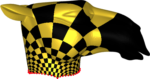
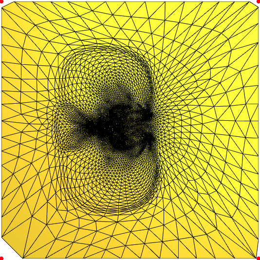
Fig. 1. Textured camel head, disc boundary vertices coloured in red (left). Parameterization onto u,v-plane (right).
Ideally the function would be modified further: the original paper authors mention that the square parametrization should split every edge in the boundary that runs around the corner of the square so that edges are mapped exactly onto the square’s boundary, rather than being distorted as an “L-shape” [4]. My code currently ignores this step, and many vertices must lie on the parameterization boundary for it to resemble a square. This is shown in the left image of Figure 1, where no edges touch the square’s corners. In summary, the fewer the boundary vertices, the less square the parameterization, and the worse it enables efficient image compression.
After the boundary of the mesh is mapped to the edges of a square domain, I use Libigl’s built-in harmonic parameterization function to generate a harmonic u,v-parameterization of my surface. This step similarly deviates from the approach suggested by “Geometry Images”: a parameterization that better-minimizes geometric stretch is recommended instead [4].
C. QUANTIZATION
The next step, following the parametrization, is quantization. This step is written completely by me, attempting to follow Gu et al.’s logic. Consequently, there is likely has a lot of room for optimization in this step.
Currently the vertices are being sampled onto the 2D image domain by searching at each point on the image grid for the which point on the mesh in terms of u, v is closest to the current pixel being sampled for the geometry image. Once the point has been chosen, its x, y, and z coordinates are quantized and scaled so that they are represented by the red, green, and blue channels of the pixel’s 24-bit RGB value, respectively.
My implementation deviates from Gu et al.’s method as well, geometry images are intended to use 16-bit colours to represent vertex positions [5] to take advantage of the fact that vertex coordinates do not need to be so precise.
In my simplified implementation, to convert the coordinates to RGB the values are simply normalized, then scaled in a way that the smallest coordinate value of the mesh is represented by 0 in one of the colour channels, and the largest by 255. All floating-point numbers are also rounded to integers at this point.
D. ENCODING
Encoding happens relatively easily: after quantization the mesh is already in its n x n representation format, where all its vertices have now been shifted so that their [x, y, z] coordinates are each in the range [0, 225]. From this point we can simply encode these directly as RGB values. The Pillow library can generate an image and save it to disk with only a few lines of code.
E. DECODING.
To decode an image and reconstruct our mesh, we simply apply the steps outlined above in reverse. In the demo I choose to leave the mesh vertex coordinates positions scaled to positions in [0, 255], since the quantization step in my algorithm only preserves vertex locations relative to each other and does not record their absolute magnitude. The original authors propose some sideband information to help with the decoding of their object [4], and this absolute magnitude could easily be included here to keep this original information at next to no cost.
V. RESULTS.
My personal goal for this project was to achieve a compression rate on a mesh object that decreased the file size, so that compression would indeed occur on my test object. On the genus-0 camel head mesh that I used for testing I achieved compression results that were significantly better than expected.
The original “camelhead.off” file, uncompressed, is 767 KB in size. The 256x256 geometry image parameterization I saved as a PNG is just 23.26 KB in size! Perhaps more surprisingly, the 32x32 image is a contained in a measly 1443 B (1.44 KB). That means my compressed files are 33 and 532 times smaller than the original file format, respectively. The geometry images and the quality of their reconstructions are visualized in Figure 2 and Figure 3 below.
I also experimented with applying textures on top of the meshes. Comparing and contrasting the checkerboard texture applied to the original mesh in Figure 1 with the texture mapped onto the compressed reconstructions in Figure 3, we can see that visually there appears to be significant distortion in the case of the 32x32 geometry image.
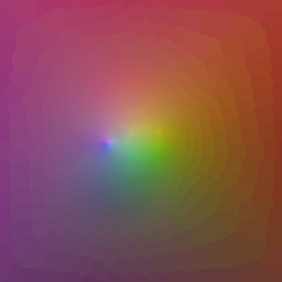

Fig. 2. 32x32 u,v-parameterization (left) and 256x256 u,v-parameterization (right)
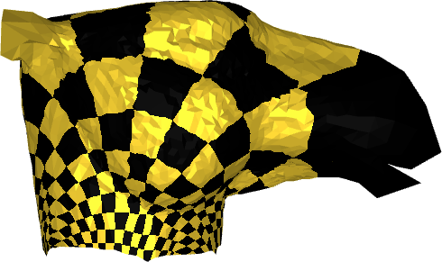
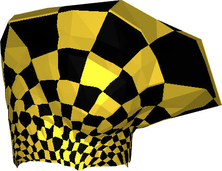
Fig 3. Textured reconstructions from 32x32 (left) and 256x256 (right) geometry images
IV. DISCUSSION.
In addition to summarizing some mesh compression strategies, I was able to achieve significant compression rates on a genus-0 mesh using a simplified method outlined in the paper “Geometry Images” by Gu et al. However, my approach has several limitations in addition to the ones outlined by the original paper.
For example, in the parameterization step, I do not minimize geometric stretch, even though a poor parameterization is known to markedly decrease the effectiveness of compression [4]. Since my implementation replaces the original geometric stretch parameterization with a harmonic parameterization, I do not take any steps to iteratively refine the cut or parameterization that I use when creating my geometry image. Similarly, I would observe higher compression rates if I were to correctly partition edges wrapping around the corners of the geometry image so that the entire u,v-domain is used in the parameterization.
As a second example, my implementation also does not cut a mesh to a topological disc. This means that I can only compress meshes which are of genus-0. In contrast, the original algorithm can compress a surface of genus-6 [4].
Lastly, further study is required to analyze how this algorithm performs in real time. The compression step does not happen in real time, because sampling each pixel value when constructing the geometry image takes too long. A cleverer implementation of this is required to achieve a real-time compression step. The decompression step, while technically real-time, currently assumes the image is already in memory. Loading the geometry image from disk would decrease decompression speeds.
REFERENCES.
[1] Wikipedia contributors, “Polygon Mesh,” Wikipedia, https://en.wikipedia.org/wiki/WebGL (accessed Dec. 11, 2023).
[2] Wikipedia contributors, “Polygon Mesh,” Wikipedia, https://en.wikipedia.org/wiki/Polygon_mesh (accessed Dec. 11, 2023).
[3] A. Maglo, G. Lavoué, F. Dupont, and C. Hudelot, “3D mesh compression,” ACM Computing Surveys, vol. 47, no. 3, pp. 1–41, 2015. doi:10.1145/2693443
[4] X. Gu, S. J. Gortler, and H. Hoppe, “Geometry images,” Proceedings of the 29th annual conference on Computer graphics and interactive techniques, pp. 355–361, Jul. 2002. doi:10.1145/566570.566589
[5] H. Hoppe and E. Praun. “Shape compression using spherical geometry images,” Advances in Multiresolution for Geometric Modelling, pp. 27–46. 2005. Doi:10.1007/3-540-26808-1_2
[6] G. Peyré and S. Mallat, “Surface compression with geometric bandelets,” ACM SIGGRAPH 2005 Papers, 2005. doi:10.1145/1186822.1073236
[7] T. Ochotta and D. Saupe, “Image‐based surface compression,” Computer Graphics Forum, vol. 27, no. 6, pp. 1647–1663, 2008. doi:10.1111/j.1467-8659.2008.01178.x
[8] K. Mamou, C. Dehais, F. Chaieb, and F. Ghorbel, “Shape approximation for efficient progressive mesh compression,” 2010 IEEE International Conference on Image Processing, 2010. doi:10.1109/icip.2010.5653218
[9] Y. Shi, B. Wen, W. Ding, N. Qi, and B. Yin, “Realistic mesh compression based on geometry image,” 2012 Picture Coding Symposium, 2012. doi:10.1109/pcs.2012.6213304
[10] A. Sinha, J. Bai, and K. Ramani, “Deep learning 3D shape surfaces using geometry images,” Computer Vision – ECCV 2016, pp. 223–240, 2016. doi:10.1007/978-3-319-46466-4_14
[11] P. Sander, S. Gortler, J. Snyder and H. Hoppe, “Signal-Specialized Parametrization,” Eurographics Symposium on Rendering, 2002.
[12] “NumPy,” https://numpy.org/ (accessed Dec. 11, 2023).
[13] Libigl, “Igl Python Bindings,” https://libigl.github.io/libigl-python-bindings/ (accessed Dec. 11, 2023).
[14] skoch9, “Meshplot,” GitHub, https://github.com/skoch9/meshplot/ (accessed Dec. 11, 2023).
[15] “Pillow,” GitHub, https://github.com/python-pillow/Pillow (accessed Dec. 11, 2023).
[16] S. Brugger. “map_vertices_to_circle.cpp,” GitHub, https://github.com/libigl/libigl/blob/main/include/igl/map_vertices_to_circle.cpp (accessed Dec. 11, 2023).