Final update: Supplemental Project Report Information
Final updates to project
You can now download the .ipynb Jupyter Notebook file I developed throughout this project and used in my project demo. It is also available through the GitHub repository for this project at /assets/download/csc461-proj-final.ipynb.
I do not have any advice on getting the notebook to run locally other than the following:
Locally I used conda to manage my environment. At the time of development I was using:
python 3.10.10igl 2.2.1meshplot 0.4.0numpy 1.25.2pillow 9.4.0pythreejs 2.4.2- whatever widgets VS Code recommended during execution
The libigl tutorial meshes may also be useful.
Details left out of the report
There were two technical details about my implementation that wanted to address in more detail outside of my report:
- Mapping the boundary around the edges of the square.
When I talked about boundary edges and vertices, I meant these ones on the “cusp” of the camel’s neck where its inside and outside meet:

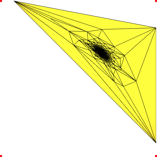
In our u,v-parameterization, these vertices and edges need to be mapped around the boundary of the unit square in order to improve it. Occassionally, when edges are mapped around the boundary of the image, an edge is mapped between two vertices on different sides of the square. This means in the parameterization the edge should appear in an “L” shape. In practice, in the parameterization the edge becomes a straight line which cuts straight through the square instead of tracing its sides. Like so:
This is fixed by splitting the edge at exactly the point a vertex would be parameterized to the corner of the square that the edge is meant to pass through, so that the original edge becomes 2 edges (one beginning from each original vertex) connected to this point. Then the “edge” correctly maps around the sides of the square. My code does not implement this edge splitting technique, but the original “Geometry Images” paper does.
- The bottleneck in my parameterization code
The bottleneck in my parameterization code occurs during the step where vertices are quantized and sampled to create my geometry image. In particular, this line:
colours[i,j] = scaled_v[np.argmin(np.linalg.norm(scaled_uv - np.array([j, i]), axis=1))]
Computes the closest point to point (i, j) on the image. However, not in a sophisticated manner: it calculates the distance from every point in the mesh to the point (i, j), and picks the nearest one.
Not only is this incredibly slow, but the number of times the line is run scales quadratically with the image dimensions. This is a major flaw with my implementation (but does allow it to produce a hacky demo).
Industry compression standards
It is worth emphasizing that to my knowledge geometry images are not currently a industry-standard compression technique. Alliez and Grotsman provide some criticisms 1:
“Despite its obvious importance for efficient rendering, this technique reveals a few drawbacks due to the inevitable surface cutting: each geometry image has to be homeomorphic to a disk [. . .] Another drawback comes from the fact that the triangle or the quad primitives of the newly generated meshes have neither orientation nor shape consistent with approximation theory, which makes this representation not fully optimized for efficient geometry compression as reflected in the rate-distortion tradeoff.”
In their feedback, Victor and Matthew mentioned alternative mesh compression strategies. One (used in industry) is Nanite, part of Unreal Engine. Nanite is comparable to geometry images in the sense that it provides level-of-detail (LOD) for models. TMF is another less popular compression method which relies on a similar technique to Nanite (an efficient mesh storage format). Many more compression implementations can also be found in the fantastic overview of current technologies written by Maglo et al. [2].
Thanks to everyone
Speaking of Victor and Matthew – a special thanks to them for keeping up with my project throughout its entire development and providing advice on the project’s direction, some library suggestions, and encouragement!
And thank you to everyone reading this. It was really sweet knowing people were (are?) paying attention to this website. I hope that you learned something about mesh compression from this project!
References
1 P. Alliez and C. Gotsman, “Recent advances in compression of 3D meshes,” Mathematics and Visualization, pp. 3–26. doi:10.1007/3-540-26808-1_1
[2] A. Maglo, G. Lavoué, F. Dupont, and C. Hudelot, “3D mesh compression: Survey, comparisons, and emerging trends,” ACM Computing Surveys, vol. 47, no. 3, pp. 1–41, 2015. doi:10.1145/2693443